
Report on the Error Control Codec Laboratory
A data transmission system
Element | Description |
Source | Generates the information to be transmitted. |
|
Source coder | Converts the source signal to a transferable signal par example does A/D-converting |
Channel coder |
Converts the signal to match the characteristics of the transmission channel. |
Channel | The media we transfer the signal through |
Channel decoder | Decodes the received signal and restores the signal encoded by the channel coder. |
Source decoder | Decodes the signal generated by the source coder and restores the source signal in a form suitable for the destination. |
Destination | Receives the information. |
The source coder and channel coder could be one block. And on the receiver side the channel decoder and the source decoder could also be one block which performs both tasks at once. But we would loose flexibility. The source coder is related to the source and matches the signal of one special source to a generic signal which could have been generated by any source. So it hides the characteristics of the source. The channel coder hides the characteristics of the channel. So we can exchange the transmission channel without changing the complete system. We just have to change channel encoder and decoder.
Error control codec
Every real channel adds noise to the transferred signal. This noise can damage our transferred data. Without any precautions the receiver would not even perceive that there was an error in transmission. So the we can apply some error correction mechanism in the channel coder and decoder to implement a virtually error free channel. The prize of error correction is redundancy which results in decreased performance for the transmission.
A (n,k) linear block
code encodes each k-bit data word in n-bit code word. The number of messages to be transferred is 2k. The number of
possible codewords is 2n. As n>k the number of codewords is larger than the number of data words. This redundancy
can be used for error detection and/or error correction.
The Hamming distance between two codewords describes the
number of different bits in the words. If a codeword is imagined as a point in a n dimensional system than the Hamming distance
is the number of steps to between two points. The distance DH of a code is the minimum of the distances between it’s
codewords. The Hamming weight of a word is the number of nonzero bits in the word.
A code of distance DH can either detect (DH -1) bits in error or correct up to (DH -1)/2 bits in error. The Distance between two codewords can be imagined as a line on which DH steps are required to get from code 1 to code 2. As long as there remains one step to the next valid codeword the distance can be used for any combination of error correction and error detection.
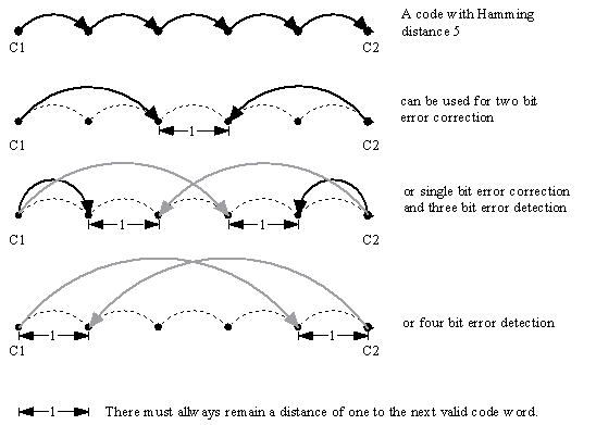
Of cause when dealing with a code the minimal distance between all codewords must be used.
Design of a (6,3) codec
dataword:
D = [D1D2D3]
codeword: C = [C1C2C3C4C
5C6] = [P1P2D1P3D2D3]
with
P
1=D1 D2
D2
P2=D1 D3
P3=D2
D3.
as C=G·D
and
C1=g11·D1 g12·D2 g13·D3
C2
=g21·D1 g22·D2 g23·D3
C3=g31·D1 g32·D2 g33·D3
C
4=g41·D1 g42·D2 g43·D3
C5=g51·D1 g52·D2 g53·D3
C6
=g61·D1 g62·D2 g63·D3
and
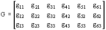
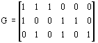
The codewords generated by this matrix are:
Data | Code |
000 |
000000 |
001 | 010101 |
010 |
100110 |
011 | 110011 |
100 | 111000 |
101 | 101101 |
110 | 011110 |
|
111 | 001011 |
The distance DH of the code is 3. The code is expected to correct one bit errors or to detect two bit errors.
The
Hamming bound for t=1:
| codeword length n = 6 |
dataword length k = 3 | |
bits in error to correct t = 1 | |
|
correct |
The decoder must calculate the parity checks on the received data bits and compare them with the receives parity bits. Assumed we received a codeword R [R1R2R 3R4R5R6] the syndrome S [S1S2S3] can be calculated as
S1 = R3 R5 R1
S2 = R3 R6 R2
S3 = R5
R6 R4
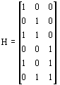
S = R · H
S1 = h11·R
1 h12·R2 h
13·R3 h14·R4 h15·R5 h16·R6
S
2 = h21·R1 h22·R2 h23·R3 h24·R
4 h25·R5 h
26·R6
S3 = h31·R1 h
32·R2 h33·R3 h34·R4 h35·R5 h36·R6
so
Electrical design
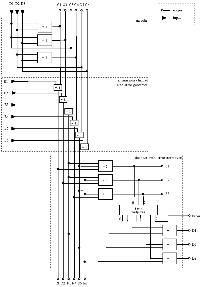
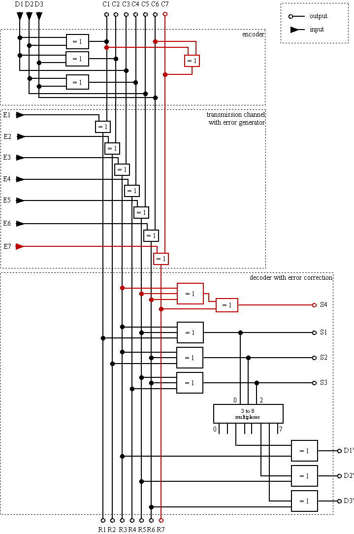
The picture shows the complete solution as assembled in the laboratory with encoder, transmission channel and decoder with automatic correction. It implements a (6,3) Hamming code with automatic one bit error correction.
Given a codeword C
and a received codeword R the syndrome S is 0 if R = C. Assuming there was an error in transmission we have R = D E.
S = (D E) · H
S = D · H E · H
we know that D · H is 0
S = E · H
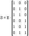
When E is a single bit error E has the form 000001 to 100000. So E just selects one row of H to be S. If we mirror H horizontally we see that any single bit error generates a syndrome which indicates the position of the bit in error in binary encoding, assumed that S1 is position 20, S2 21 and S3 22. If we feed this in a 3 to 8 multiplexer we just have to perform an exclusive or on the received codeword and the output of the multiplexer to get the corrected code word.
Detecting two bit errors
For a code which is which is able to detect two-bit errors an correct single-bit
errors we need a Hamming distance of 4. As the distance of the (6,3) code is 3 we have to add another parity check bit P
4 = D1 D2 D3.
As the generator matrix G just maps the three bit codeword to the 7 bit data word we can modify G(6,3) by adding another column.
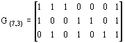
Some modification must be applied to H.
S1 = R3 R5 R1
S2 = R3 R6 R2
S3 = R5
R6 R4
S4 = R5 R6 R4
R7
S = R · H
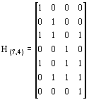
The codewords would remain the same except for an additional bit at the end.
Data | Code |
000 | 0000000 |
001 | 0101011 |
010 | 1001101 |
011 | 1100110 |
100 |
1110001 |
101 | 1011010 |
110 | 0111100 |
111 | 0010111 |
The Hamming distance of the new code is 4
The circuit design of the new code looks like this:
Laboratory protocol
When assembling the designed circuit in the laboratory there were some changes.
The generated codewords matched the designed codewords.
The decoder
decoded the transferred data correctly.
Table of all single bit errors.
It must be remembered that we used the least
significant bit as first bit. So to see that S gives the position of the bit in error we must mirror S horizontally.
D [D1 D2D3] | C | E |
R |
S |
D’ |
000 | 000000 | 000001 | 000001 | 011 | 000 |
000 |
000000 | 000010 | 000010 | 101 | 000 |
000 | 000000 | 000100 | 000100 | 001 |
000 |
000 |
000000 | 001000 | 001000 | 110 | 000 |
000 | 000000 | 010000 | 010000 | 010 | 000 |
000 | 000000 |
100000 | 100000 | 100 | 000 |
001 | 010101 | 000001 | 010100 | 011 | 001 |
001 | 010101 | 000010 | 010111 | 101 | 001 |
001 | 010101 |
000100 | 010001 | 001 | 001 |
001 | 010101 | 001000 | 011101 | 110 | 001 |
001 | 010101 | 010000 | 000101 | 010 | 001 |
001 | 010101 | 100000 | 110101 | 100 | 001 |
.
.
.
111 | 001011 | 000001 | 001010 | 011 | 111 |
111 | 001011 | 000010 | 001001 | 101 |
111 |
111 |
001011 | 000100 | 001111 | 001 | 111 |
111 | 001011 | 001000 | 000011 | 110 | 111 |
111 | 001011 |
010000 | 011011 | 010 | 111 |
111 | 001011 | 100000 | 101011 | 100 | 111 |
All 2 bit errors for the arbitrary chosen data word D=001 !’ C=010101
D [D1D2D 3] | C | E | R |
S | D’ |
001 | 010101 | 000011 | 010110 | 110 |
110 |
001 |
010101 | 000101 | 010000 | 010 | 000 |
001 | 010101 | 000110 | 010011 | 100 | 011 |
001 | 010101 |
001001 | 011100 | 101 | 110 |
001 | 010101 | 001010 | 011111 | 011 | 110 |
001 | 010101 | 001100 | 011001 |
111 | 101 |
001 | 010101 | 010001 | 000100 | 001 | 000 |
001 | 010101 | 010010 | 000111 | 111 | 011 |
001 |
010101 | 010100 | 000001 | 011 | 000 |
001 | 010101 | 011000 | 001101 | 100 | 101 |
001 | 010101 | 100001 | 110100 | 111 | 000 |
001 |
010101 | 100010 | 110111 | 001 | 011 |
001 | 010101 | 100100 | 110001 | 101 | 011 |
001 | 010101 |
101000 | 111101 | 010 | 101 |
001 | 010101 | 110000 | 100101 | 110 | 101 |
The marked errors can be detected because they result in an unused value for S. This results from some of the codewords having a Hamming distance of four. We can indicate these errors using the output 7 of the 3 to 8 multiplexer.
The next table shows all single and two bit errors for (7,3) codec, D=000 and an arbitrary chosen dataword to prove that 000 has no special behaviour.
D [D1D2D3] | C | E | R | S | D’ |
000 | 0000000 | 0000001 | 0000001 | 0001 | 000 |
000 | 0000000 | 0000010 | 0000010 | 0111 | 000 |
000 | 0000000 | 0000100 | 0000100 | 1011 | 000 |
000 | 0000000 | 0001000 | 0001000 | 0010 | 000 |
000 | 0000000 | 0010000 | 0010000 | 1101 | 000 |
000 | 0000000 | 0100000 | 0100000 | 0100 | 000 |
000 | 0000000 | 1000000 | 1000000 | 1000 | 000 |
000 | 0000000 | 0000011 | 0000011 | 0110 | 000 |
000 | 0000000 | 0000101 | 0000101 | 1010 | 000 |
000 | 0000000 | 0000110 | 0000110 | 1100 | 111 |
000 | 0000000 | 0001001 | 0001001 | 0011 | 000 |
000 | 0000000 | 0001010 | 0001010 | 0101 | 001 |
000 | 0000000 | 0001100 | 0001100 | 1001 | 010 |
000 | 0000000 | 0010001 | 0010001 | 1100 | 000 |
000 | 0000000 | 0010010 | 0010010 | 1010 | 111 |
000 | 0000000 | 0010100 | 0010100 | 0110 | 111 |
000 | 0000000 | 0011000 | 0011000 | 1111 | 100 |
000 | 0000000 | 0100001 | 0100001 | 0101 | 000 |
000 | 0000000 | 0100010 | 0100010 | 0011 | 001 |
000 | 0000000 | 0100100 | 0100100 | 1111 | 010 |
000 | 0000000 | 0101000 | 0101000 | 0110 | 001 |
000 | 0000000 | 0110000 | 0110000 | 1001 | 100 |
000 | 0000000 | 1000001 | 1000001 | 1001 | 000 |
000 | 0000000 | 1000010 | 1000010 | 1111 | 001 |
000 | 0000000 | 1000100 | 1000100 | 0011 | 010 |
000 | 0000000 | 1001000 | 1001000 | 1010 | 010 |
000 | 0000000 | 1010000 | 1010000 | 0101 | 100 |
000 | 0000000 | 1100000 | 1100000 | 1100 | 100 |
010 | 1001101 | 0000001 | 1001100 | 0001 | 010 |
010 | 1001101 | 0000010 | 1001111 | 0111 | 010 |
010 | 1001101 | 0000100 | 1001001 | 1011 | 010 |
010 | 1001101 | 0001000 | 1000101 | 0010 | 010 |
010 | 1001101 | 0010000 | 1011101 | 1101 | 010 |
010 | 1001101 | 0100000 | 1101101 | 0100 | 010 |
010 | 1001101 | 1000000 | 0001101 | 1000 | 010 |
010 | 1001101 | 0000011 | 1001110 | 0110 | 010 |
010 | 1001101 | 0000101 | 1001000 | 1010 | 010 |
010 | 1001101 | 0000110 | 1001011 | 1100 | 101 |
010 | 1001101 | 0001001 | 1000100 | 0011 | 010 |
010 | 1001101 | 0001010 | 1000111 | 0101 | 011 |
010 | 1001101 | 0001100 | 1000001 | 1001 | 000 |
010 | 1001101 | 0010001 | 1011100 | 1100 | 010 |
010 | 1001101 | 0010010 | 1011111 | P>1010 | 101 |
010 | 1001101 | 0010100 | 1011001 | 0110 | 101 |
010 |
1001101 | 0011000 | 1010101 | 1111 | 110 |
010 | 1001101 | 0100001 | 1101100 | 0101 | 010 |
010 | 1001101 | 0100010 | 1101111 | 0011 | 011 |
010 | 1001101 | 0100100 | 1101001 | 1111 | 000 |
010 | 1001101 | 0101000 | 1100101 | 0110 | 011 |
010 | 1001101 | 0110000 | 1111101 | 1001 | 110 |
010 | 1001101 | 1000001 | 0001100 | 1001 | 010 |
010 | 1001101 | 1000010 | 0001111 | 1111 | 011 |
010 | 1001101 | 1000100 | 0001001 | 0011 | 000 |
010 | 1001101 | 1001000 | 0000101 | 1010 | 000 |
010 | 1001101 | 1010000 | 0011101 | 0101 | 110 |
010 | 1001101 | 1100000 | 0101101 | 1100 | 110 |
Analysing the values of S for the new code we can see that
An error detection circuit has to calculate.
| not
zero | even | ||
| Err = |  |  |
(S1S2S3S4) |
We have to exclude zero from the set of even numbers.
This results a circuit for indicating non recoverable errors to be:
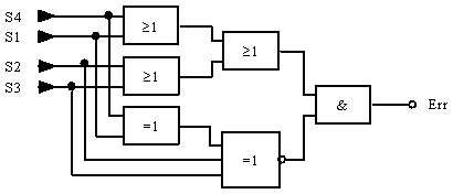
Err is set to one if an 2 bit Error was detected. One bit errors are still corrected because S (6,3) consisting of [S1S2S3] will be handled by the 2 to 8 multiplexer. The new error E=0000001 results in S(6,3) being 000. But as the error is in R7 the data bits are unchanged.


